The Robot and the Simulation
In Chapter 1, we watched the high-level policy guide the robotic arm to locate, grasp, and deposit a colored cube into a bin. To the policy's neural network, the physical world is treated largely as an abstract space of incremental commands: request a displacement in Cartesian coordinates , adjust the wrist heading , and modulate the gripper jaws.
In physical reality—and inside the MuJoCo simulation that mirrors it—a robot cannot glide through space by wishing to be somewhere else. An industrial manipulator is an intricate multi-body mechanical assembly: cast-aluminum castings, high-torque brushless DC motors, harmonic drive gearboxes, high-resolution optical encoders, and rubberized gripping pads interacting with objects through contact mechanics and friction.
To bridge the gap between high-level policy intentions and low-level physical dynamics, the manipulation system operates across three tightly coupled levels of control running at distinct frequencies:
| Level | Subsystem | Frequency | Period | Primary Function |
|---|---|---|---|---|
| High Level | The Policy (Brain) | Evaluates camera feeds and language prompt; emits incremental Cartesian displacements and target jaw opening. | ||
| Middle Level | The Controller | Converts Cartesian requests into target joint angles via inverse kinematics; enforces velocity, acceleration, and workspace safety limits. | ||
| Low Level | Motors & Physics Engine | MuJoCo computes multi-body dynamics, contact manifolds, friction cones, and actuator PD torques driving joints toward setpoints. |
The low level is where physical reality is decided. Here, the simulator solves the master equation of motion for the robot's physical body:
In plain English, with zero math jargon, this formula simply states:
Motor Push = Effort to Accelerate + Rotational Fling + Gravity Drag + Outside Pushback
Whenever the arm moves, its motors must fight against four physical forces:
- Accelerating Heavy Metal (): Heavy metal parts resist speeding up or slowing down. When the arm is outstretched horizontally like a broomstick, it takes much more muscle to start swinging it than when it is tucked in close.
- Rotational Fling and Swerve (): When the arm spins fast, its links want to fling outward (like riding a fast carousel). If the shoulder swings while the elbow reaches out, the two motions push each other sideways.
- Gravity Drag (): The constant downward pull of the Earth trying to drag the heavy arm down toward the floor.
- Outside Pushback (): Whenever the hand presses on the table, bumps a bin rim, or pinches a cube, that contact push at the fingertips travels all the way back up the arm and twists the motors.
To make the arm move, the motors must push () hard enough to speed up the metal, fight the spin, beat gravity, and overcome anything the hand is touching. (The full mathematical derivation of each matrix is detailed in Appendix A.)
Here's a two-link arm running that exact equation live. The equation at the top is the control panel, and the bars on the right show how much torque each term asks for at each joint.
Figure 2.1 Interactive two-link arm running the manipulator equation live. The equation at the top toggles physical terms on and off, while real-time torque bars display joint efforts.
Things to try, one term at a time:
- (motors): Click it off. The arm goes limp and gravity wins. Click it back on and the motors hold whatever pose the arm is in. At rest, the blue bar exactly cancels the amber one, which is what "holding still" costs.
- (gravity): Turn it off with motors off and the arm floats like it's in orbit. Turn it on and notice the gravity bar changes with the pose: big when the arm is stretched out sideways, near zero when it hangs straight down.
- (inertia): Slide the payload up. The same pull now gives less acceleration. It also depends on pose: a stretched arm is harder to swing than a folded one.
- (Coriolis and centrifugal): Turn off motors and gravity, then hit "Give it a spin". The green bar only wakes up when the arm is moving, because it is the joints throwing each other around. Turn it off mid-spin and the motion goes visibly wrong.
- (outside push): Drag on the canvas. Your pull is a force at the hand, and turns it into joint torques. Pull along a straight arm and the bars barely move; pull sideways and they jump.
The line under the bars shows the left and right sides of the equation staying equal the whole time.
Modeling note: Real robot joints experience mechanical friction that dissipates energy and brings moving parts to rest. To keep the playground intuitive without introducing a sixth term to the equation, a small amount of viscous joint damping is included and accounted for within the motor torque () bar.
Why Contact Simulation Is the Hardest Part
In free space (where the hand touches nothing, so ), computing the robot's motion is mathematically straightforward: one can invert the mass matrix to solve for joint accelerations:
and integrate forward in time using standard numerical integration.
In robotic manipulation, however, the arm is almost never in free space: the entire task requires making and maintaining physical contact with objects. Contact dynamics introduces severe non-linear constraints:
- Non-penetration constraints: Rigid bodies cannot occupy the same volume in space (distance , normal contact force , with complementary condition ).
- Coulomb friction cones: Gripper finger pads can only exert tangential shear force up to the boundary of the friction cone (). If tangential force exceeds this limit, the object slips.
Rather than modeling contacts as crude spring-damper penalty forces that vibrate and destabilize numerical integration, MuJoCo formulates contact dynamics as a convex optimization problem (a linear complementarity problem) solved 500 times per second ( timestep). At every tick, it determines the exact contact impulses that prevent penetration while satisfying friction cone limits.
From these calculated forces, the simulator determines what physically happens: Does the hand reach the cube? Does the cube tilt or slip out of the jaws? Can the silicone friction pads sustain the vertical load when the arm lifts? The low level answers these existential physical questions.
Before we examine how the controller mediates these forces, we must first understand the robot's physical anatomy and how its geometry is represented.
2.1 Six Joints and Two Jaws
We begin with the physical components of the manipulation cell. The hardware consists of two primary mechanisms: an articulated robotic arm and a parallel-jaw gripper.
The arm is a Universal Robots UR5e, one of the most widely used collaborative robots in industrial manufacturing and robotics research. Our simulated model is a high-fidelity digital twin that mirrors the exact link lengths, joint limits, inertial tensors, and actuator dynamics of the physical machine.
Figure 2.2 The simulated UR5e manipulation cell at the moment of grasping. Joints 1 through 6 form an open serial kinematic chain from the stationary base to the tool flange. The cell includes an OnRobot RG6 two-jaw gripper, a wrist-mounted camera, and an overhead camera mounted on an extruded-aluminum stand.
The UR5e is an open serial kinematic chain featuring six revolute (rotational) joints:
- Joint 1 (Base): Rotates the entire arm about the vertical Z-axis ().
- Joint 2 (Shoulder): Pitches the upper arm forward and backward ().
- Joint 3 (Elbow): Pitches the forearm relative to the upper arm ().
- Joint 4 (Wrist 1): Pitches the wrist assembly up and down ().
- Joint 5 (Wrist 2): Yaws the tool flange left and right ().
- Joint 6 (Wrist 3): Rolls the tool mounting plate about the tool axis ().
The arm contains no prismatic (sliding or telescoping) joints. No link can expand or contract. Every movement of the hand across the 3D workspace is produced purely through the coordinated rotation of these six revolute axes.
Mounted to the tool flange of Wrist 3 is the end-effector: an OnRobot RG6 parallel gripper. The gripper consists of two opposing fingers driven synchronously by an internal motor. The distance between the finger pads—the jaw gap—can vary continuously from (fully closed) to (fully open). This single degree of freedom is the only action the gripper can perform.
Consequently, the complete physical configuration of the robot is described by exactly seven scalar values: six joint angles and one jaw gap:
where denote the joint angles and denotes the jaw separation.
Figure 2.3 provides an interactive 3D model of the robot rendered directly from this 7-dimensional configuration vector. You can manipulate each slider to see how individual joint rotations alter the arm's shape, drag the canvas to rotate the 3D view, or use the jump buttons to load configurations recorded during an autonomous pick-and-place trial.
Figure 2.3 Interactive 3D visualization of the robot's 7-dimensional configuration space. The numbered circles correspond to the six revolute joints from Figure 2.2. The arm links match the exact physical dimensions of the UR5e. Adjust the sliders to explore joint limits, or click the preset buttons below to load key poses from a recorded episode.
Beyond its motors, the robot relies on two complementary sensor systems to perceive the cell and monitor its own state:
- Proprioceptive Sensing: Optical rotary encoders mounted on each motor shaft measure the joint angles with sub-milliradian precision. Hall sensors inside the gripper track the jaw gap .
- Visual Sensing (Dual Cameras):
- Static Overhead Camera (
cam_static): Positioned on an elevated extruded-aluminum frame overlooking the workspace. It delivers a wide-angle global view () capturing the entire table, the colored objects, and the two sorting bins. - Wrist-Mounted Camera (
cam_wrist): Attached directly to Wrist 3 just above the gripper palm. It provides an egocentric, high-resolution perspective looking down past the fingers. As the arm descends toward an object, this in-hand view resolves fine spatial alignment and prevents self-occlusion by the robot's own links.
- Static Overhead Camera (
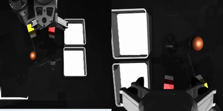
Figure 2.4 The simultaneous camera streams provided to the policy at step 140. Left: The fixed overhead camera provides global context, showing the arm, tabletop clutter, and target receptacles. Right: The wrist camera peers directly down through the gripper jaws, providing close-up visual feedback essential for grasping millimeter-scale objects.
2.2 Forward Kinematics: How the Robot Localizes Its Hand
To pick up an object from the table, the robot must position its gripper jaws directly around the target. This requires knowing the exact position and orientation of the hand in 3D space at every instant.
It is tempting to assume that an external sensor measures this Cartesian position directly—such as a GPS unit or an optical motion capture system tracking the gripper's coordinates. In standard industrial robotics, however, robots have no onboard sensor that directly measures Cartesian tool coordinates, nor do they rely on external optical tracking during routine operation. External optical trackers are costly, susceptible to line-of-sight occlusions, and difficult to maintain reliably in cluttered factory environments.
The robot measures only the angular positions of its six joints through internal optical encoders. To determine where its hand is located in the physical room, the robot must compute the position using the known geometry of its mechanical links.
This computation is called forward kinematics (FK). In plain English, it answers a single question:
"If my joints are set to these angles, where is my hand in the room?"
Because the robot's metal links never stretch or bend, each joint acts like a leg of a mechanical compass:
- The base turns the arm left or right.
- The shoulder pitches the upper arm up or down.
- The elbow extends the forearm forward.
- The three wrist joints orient the gripper.
Chaining these rotations one by one from the base pedestal to the fingertips gives the exact 3D position and orientation of the gripper:
Intuition: The Planar 2-Link Arm
To see how this works without getting tangled in 3D rotation matrices, look at the arm from the side as a simple two-link mechanism (shoulder and elbow):
- Elbow position: Start at the shoulder and step outward along the upper arm () at angle .
- Wrist position: Start at the elbow and step outward along the forearm () at angle .
- Hand position: Hangs straight down below the wrist by the tool length ().
In elementary trigonometry:
Because our pick-and-place task maintains the gripper in a downward-pointing orientation perpendicular to the tabletop, the hand position is simply shifted downward from the wrist by the tool length:
Figure 2.5 illustrates this planar kinematic model. Moving the shoulder and elbow sliders updates the arm's posture in real time, immediately recalculating and displaying the Cartesian position of the hand.
Figure 2.5 A side view of the UR5e arm drawn to true scale. The upper arm is 425 mm and the forearm is 392 mm. The dashed rectangle indicates the permissible workspace volume above the tabletop. The wrist joints are held fixed so the gripper always points downward. Move the sliders to test forward kinematics, or click the preset buttons to inspect typical operational postures.
The Uniqueness of Forward Kinematics
Notice a fundamental mathematical property of forward kinematics:
Forward kinematics is a well-posed, single-valued function. Given any valid set of joint angles , there is exactly one corresponding hand position .
There is never ambiguity, multiple branches, or uncertainty in forward kinematics. It answers the question:
"Given these joint angles, where is the hand located?"
Because it consists of simple algebraic trigonometric multiplications, forward kinematics evaluates in fractions of a microsecond on modern hardware. The simulator and robot controller execute this calculation on every single cycle to monitor hand position, detect potential collisions, and project synthetic camera viewpoints.
However, when the robot needs to perform physical work—such as moving its gripper to grasp an object detected at coordinates —it faces the inverse problem:
"Given where the hand needs to go, what joint angles will place it there?"
As we will see next, calculating this reverse mapping is much harder.
2.3 Inverse Kinematics: Going from Hand Position to Joint Angles
Forward kinematics answers the question: "The joints are at these angles; where is the hand?" As we saw in Section 2.2, this is easy to calculate because each set of joint angles gives only one single hand position.
When the robot works in the real world, however, the problem is reversed. A camera or AI policy detects a target cube at 3D position on the table. To move the gripper to the cube, the controller must solve the reverse question:
"I need my hand at . What joint angles will put it there?"
This calculation is called inverse kinematics (IK). Unlike forward kinematics, inverse kinematics is non-linear, mathematically difficult, and often has multiple different answers.
The Two Main Challenges: Zero Answers or Many Answers
When you calculate joint angles from a desired 3D hand position, two physical problems happen:
1. Unreachable Targets (Zero Answers)
If a target is too far away—beyond the full reach of the arm ()—or too close to the body, no joint angles can possibly reach it.
Try this in Figure 2.5 above: drag the hand far away toward the canvas edge. As soon as you drag outside the arm's reach, the sliders stop moving. The math becomes impossible (trying to calculate where ).
2. Multiple Kinematic Solutions (Many Answers)
Even when the arm can reach a target, there is rarely just one way to touch it.
Think about the two-link arm on a flat table. We use the law of cosines on the triangle formed by the shoulder, elbow, and hand to find the elbow angle :
Because cosine is symmetrical (), this equation gives two valid mathematical answers:
The positive angle produces the elbow-down pose (elbow bending forward). The negative angle produces the elbow-up pose (elbow bending backward).
You can see both answers in Figure 2.5:
- Look at the faint dashed outline: its hand is at the exact same point as the solid arm, but its elbow bends in the opposite direction.
- Click "bend the elbow the other way": the hand stays completely still while the arm links swing around it.
The Physical Dangers of Multiple Solutions
In pure math, both elbow poses reach the target equally well. In the physical robot cell, however, they are not equally safe:
- Crashing into the Table: In Figure 2.5, drag the hand close to the table surface and click "bend the elbow the other way". One pose holds the arm safely in the air, but the other pose forces the elbow straight into the table (). On a real robot, choosing the wrong solution causes a bad physical crash against the table or safety glass.
- Sudden Jumps (Discontinuities): A full 6-axis industrial arm like the UR5e does not have just 2 solutions—it has up to 8 distinct mathematical solutions for a single 3D hand pose: If a robot controller suddenly switches from one solution to another while moving, the arm will whip (swing violently) across the cell. This triggers safety shutoffs, strains the motors, or tears the electrical cables running through the robot's joints.
Figure 2.6 lets you see all 8 mathematical solutions in 3D for the real UR5e arm. The controller needs to place the gripper on the target cube at .
Notice the faint dashed lines: all seven other arm poses start at the robot base and meet at the exact same target point. Use the three switches or the 8-button grid below to test each configuration:
- The Wrist Flip ( total joint turn): Inverting the wrist angle () forces joint 4 and joint 6 to turn by to keep the hand pointing the same way. While the gripper jaws stay completely still, the wrist joints turn by a massive in total. On a physical arm, this extreme turn winds and twists the internal power and sensor cables dangerously.
- The Elbow Down Crash ( below the table): Bending the elbow downward forces the heavy upper arm link to plunge 48 mm below the table surface. On physical hardware, this causes a severe crash that damages the robot gears and table.
- Reaching Backward with the Shoulder ( turn): Turning the shoulder base around makes the arm reach backward over its own mounting base. This swings large metal links across the entire workspace at high speed.
Figure 2.6 Interactive 3D visualization of the 8 inverse kinematic solutions of the UR5e for a locked hand pose. The target marker is locked at the target cube. Faint dashed lines show the seven other poses starting from the robot base and meeting at the gripper jaws. Toggling the shoulder, elbow, or wrist shows how mathematically identical hand positions can cause table crashes (elbow-down) or massive cable twists (wrist flip ). Drag the canvas to rotate the 3D view.
Why the AI Policy Avoids Global Inverse Kinematics
This issue explains why modern robot learning policies almost never output global joint angles directly from camera images.
If a neural network had to predict absolute joint angles, it would face a confusing choice: both elbow-up and elbow-down poses reach the target. When a network tries to average two good answers, it produces an invalid pose right in the middle that misses the target completely!
Instead, our policy works at Level 1, asking only for small, step-by-step Cartesian hand movements:
Rather than solving the complicated 8-solution inverse kinematics from scratch on every step, the low-level controller uses local differential kinematics with the robot's Jacobian matrix :
By calculating small joint angle changes along the current pose using the Jacobian pseudoinverse , the robot moves smoothly and safely from step to step without ever jumping between different solutions.
In the next section, we examine the middle-level controller that manages these movements: how it smooths sudden commands, enforces safety limits, and powers the joint motors.
2.4 The Middle Level: Smoothing, Safety Limits, and Motor Torques
In Sections 2.2 and 2.3, we solved the kinematic geometry of the cell: given a small desired Cartesian displacement , the controller calculates the corresponding joint angle adjustments .
In an ideal mathematical world, the robot would jump to those angles instantaneously. In the physical cell, however, commands cannot be applied directly to motors without intermediate safety processing. Motors have inertia, gear limits, and finite torque; cables can catch, and neural networks can occasionally request abrupt, jagged commands.
To protect the physical hardware and ensure smooth, continuous motion, the system mediates every movement through a middle-level controller running at ( period), which feeds torque setpoints into a low-level motor PD loop running at ( period).
2.4.1 What Happens to a Policy Command (100 Hz Loop)
Every , the high-level policy evaluates camera images and emits an incremental displacement command. During the subsequent window, the middle-level controller executes ten control ticks ( each). On every tick, it performs three operations:
Exponential Smoothing (Low-Pass Filter): To prevent jerky starts and stops, the raw step request is passed through a first-order low-pass filter: where sets the smoothing strength. In our simulation, (smoothing factor of ), whereas the physical UR5e arm uses stronger smoothing (, factor ) to minimize mechanical vibration.
Rate Clamping (Speed Cap): Even if the policy demands a large sudden leap—such as asking for in one step—the controller imposes a hard cap: Any displacement request exceeding this threshold is truncated and permanently discarded. Demanding an overly large step does not make the arm travel faster; it simply throws away part of the command.
Workspace Boundary & Discontinuity Guard: The controller verifies that the proposed hand target stays strictly within the authorized safe workspace box (, inside table boundaries). Furthermore, if the differential inverse kinematics solver requires any joint to turn faster than its maximum allowable velocity threshold, the controller refuses the step entirely and logs a streamer fault.
Figure 2.7 illustrates what happens to a single policy command over its ten control ticks. Adjust the requested step size and smoothing sliders to observe how rate clamping and low-pass filtering shape the motion.
Figure 2.7 Interactive inspection of the middle-level exponential filter over ten control ticks ( each). Top: Cumulative hand target motion (raw linear request vs. filtered curve). Bottom: Per-tick filter output and dispatched displacement clamped at the safety ceiling.
Two key takeaways emerge from Figure 2.7:
- Smoothing creates a small lag: Under our standard setting (), a single command delivers approximately of its requested distance over the first ten ticks, with the remainder trailing into the next window. Under the physical robot's heavier setting (), approximately is delivered immediately. This intentional lag prevents infinite acceleration spikes.
- The clamp discards extreme requests: Above per command, every tick hits the ceiling. If a policy asks for , more than half of the requested distance is discarded.
2.4.2 How Motors Follow Targets: The 500 Hz PD Loop
Once the middle-level controller computes target joint angles , the physical actuators must track those setpoints. At the low level (, timestep), MuJoCo calculates joint torques using a Proportional-Derivative (PD) control law:
where is the target setpoint, is the current joint angle, is the current angular velocity, and is the actuator torque.
- Proportional Gain ( — The Spring): Generates an active restoring torque proportional to the angular tracking error . It acts like an active torsional spring pulling the link toward the setpoint.
- Derivative Gain ( — The Damper / Brake): Opposes joint velocity (), acting like a viscous shock absorber that dissipates kinetic energy and halts oscillatory ringing.
In our digital twin, the actuator gains match the physical UR5e joints:
- Base, Shoulder, and Elbow (Large Joints): , , with a hard torque ceiling of .
- Wrists 1, 2, and 3 (Small Joints): , , with torque limited to .
Figure 2.8 isolates the elbow joint of the UR5e as it tracks a step ramp over . The simulation accounts for true link rotational inertia (), gravitational torque (), and motor torque saturation ().
Figure 2.8 Real-time simulation of the UR5e elbow joint tracking a 10° displacement ramp in 0.2 s under PD motor control. Top: Target setpoint (dashed) versus actual angular position (solid). Bottom: Actuator torque output, clamped at the motor limit of 150 N·m.
Notice three crucial behaviors illustrated in Figure 2.8:
- Inertial Motor Lag: Even with stiff gains and nominal damping (), the elbow lags approximately behind the moving target at the moment the setpoint ramp finishes (). The joint reaches of the target angle only after . The physical hand always arrives slightly after the controller commands it.
- The Danger of Insufficient Damping: Click "no braking" (). Without derivative damping to bleed off kinetic energy, the joint rings and oscillates violently around the setpoint like an undamped pendulum. Adding proper damping () brings the damping ratio , suppressing overshoot entirely.
- Gravity Sag (Steady-State Droop): At nominal stiffness (), the joint never settles perfectly on ; it comes to rest approximately below target. Damping () has zero effect on this resting droop because the arm is stationary (). Because a PD controller possesses no integral term (), the proportional spring must remain slightly stretched () to produce exactly of upward torque to support the forearm against gravity.
Lesson. Side Note: Why an Integral Term () Eliminates Sag (and why RL pipelines omit it)
In classical PID control, steady-state droop is eliminated by adding an Integral term (). Because the residual error persists over time, the accumulated integral builds upward torque until it produces the exact required to balance gravity, driving steady-state sag to . You can test this live in Figure 2.8 by adjusting the optional slider or clicking "+ integral gain".
Why do modern robot learning pipelines keep (pure PD)?
- Integral Windup: If the gripper presses against the table or contacts a bin wall during a policy rollout, the integrator continues accumulating error, ramping motor torque up to dangerous ceiling limits. When the obstacle clears, the arm snaps violently.
- Phase Lag & Overshoot: Integration introduces phase lag, reducing stability margins during rapid multi-joint trajectory tracking.
Instead of integral terms, industrial robot cells either run model-based feedforward gravity compensation () or allow the high-level policy neural network to naturally absorb the predictable actuator droop.
2.4.3 Why Sim-to-Real Fidelity Requires This Pipeline
It is tempting to simplify robot learning by letting the neural network bypass both the middle-level controller and the motor PD loop—commanding joint angles or torques directly.
In practice, doing so breaks sim-to-real transfer:
- If a policy trains in simulation without command smoothing, it learns to emit high-frequency, twitchy commands. When deployed on the physical robot, the real industrial controller clamps, filters, or safety-trips on those motions, causing the robot to fail.
- If a policy trains without realistic actuator lag and gravity droop, it expects the gripper to be where it commanded it immediately, causing it to close its fingers before the hand has physically reached the cube.
By enforcing the exact same controller code
(StreamerCore), rate clamps
(),
and joint PD dynamics in MuJoCo as on the physical robot cell, any
policy trained or evaluated in simulation transfers seamlessly to the
physical machine.
With the physical cell, its geometry, and its three control tiers fully defined, we now have a complete mathematical model of our manipulation environment. In Chapter 3, we put this system to work: writing a hand-crafted expert policy to prove that the task can be solved autonomously and reliably.