Robotics · Reinforcement Learning · Vision-Language-Action
Teaching a UR5e to Pick and Place: From Broken Rewards and 0% RL to a 50/50 Vision-Language-Action Policy
We built the simulation half of a sim-to-real robotic pilot: a UR5e arm with an OnRobot RG6 gripper learning to pick up cubes and balls and place them into bins. Along the way, RL from scratch collapsed to 0%, dense rewards paid the robot to stand still forever, DAgger trained on an anti-policy, and sophisticated generative heads lost to plain MSE. Here is how a geodesic potential field, a backplay curriculum, and online PPO on top of a 3.5B open-weights VLA took the robot from zero to a perfect 50/50 held-out success rate — even under camera blur, low light, and visual noise.
01The task and the simulated cell
The goal of this pilot is sim-to-real robotic manipulation: train policies in a physically accurate simulation, calibrate them against real teleoperation logs, and deploy them onto an industrial arm without hardware surprises.
The workcell consists of a 6-DOF Universal Robots UR5e industrial arm
equipped with an OnRobot RG6 parallel-jaw gripper mounted over a worktable.
On the table sit four randomized objects (two 45 mm cubes: red_cube,
yellow_cube, and two 50 mm spheres: blue_ball,
brown_ball) alongside two destination bins (left and right).
In each episode, the robot is instructed to pick up one specific target object and deposit it into a target bin, communicated as a natural language command:
info["instruction"] = "put the red cube in the left bin"Sim-to-real rule: actions pass through the real controller
Many simulation benchmarks let policies output direct joint positions or raw torques.
We explicitly rejected that. In this cell, every single policy action passes through
StreamerCore — the exact same C++/Python Cartesian servoing controller that
drives the physical UR5e in the laboratory.
| Layer | Frequency | Function |
|---|---|---|
| Policy action | 10 Hz | One action step = 0.1 seconds of robot time |
| Robot controller | 100 Hz | Smooths deltas, damps singularities, checks kinematic limits |
| MuJoCo physics | 500 Hz | Exact contact dynamics, 5 physics substeps per controller tick |
Because actions are executed via the robot's real controller, the robot's hardware speed limit (clamped between 0.05 m/s and 0.25 m/s) is preserved in simulation. Any policy that succeeds here produces commands the physical robot can immediately accept.
Observations: privileged state vs. raw pixels
The observation space is controlled by independent flags in envs/observation.py:
- Proprioceptive state (13 numbers): 6 arm joint angles, gripper jaw opening width, and 6D tool center point (TCP) Cartesian position and Euler orientation.
- Privileged task state (7 numbers): Target object XYZ position, orientation yaw, and target bin XYZ position. Available only to simulation-only baselines.
- Vision: Two calibrated RGB cameras matching real Intel RealSense D435i sensors — an overhead static view (
cam_static, 320×240) and an in-hand wrist view (cam_wrist, 320×240). - Language: The raw text instruction string, consumed directly by tokenizers in vision-language-action models.
02The perils of dense rewards: why RL failed first
Before training complex vision models, we asked a fundamental question: can a standard reinforcement learning agent learn this task from scratch using a state observation of 20 numbers?
Our first attempt used Soft Actor-Critic (SAC) with a textbook shaped dense reward: rewarding the negative Euclidean distance from the gripper to the object, adding a bonus for holding the object, and rewarding proximity from the object to the target bin.
We trained for 300,000 environment steps on both fixed and randomized scenes. The results were baffling:
| Experiment | Env Steps | Eval Return | Success Rate |
|---|---|---|---|
| SAC dense (fixed scene) | 300k | 116 → 512 | 0% (0/20) |
| SAC dense (randomized scene) | 300k | 137 → 403 | 0% (0/20) |
The policy's evaluation return climbed steadily throughout training, but the actual task success never budged from 0%. When we printed the commanded actions over time, we uncovered what the agent had actually learned:
step   dx     dy     dz    dyaw   grip   | TCP moved (mm)
  40  [-0.19 -0.16 -0.74  0.40  0.18]  |  81.9 mm
 100  [-0.01 -0.00 -0.50 -0.01  0.11]  |   4.0 mm
 140  [-0.00 -0.00 -0.50 -0.00  0.13]  |   0.1 mm
 280  [-0.00 -0.00 -0.50 -0.00  0.13]  |   0.0 mm (frozen)
By step 140, the policy outputs a constant vector: press down with moderate force, keep the gripper half open, and never move again for the remaining 660 steps of the episode!
The arithmetic trap
The reward function was causing this perverse incentive, not the algorithm. The reaching term was defined as:
r_reach = 1.0 - tanh(5.0 * distance_to_object)
Hovering right next to the object paid approximately 0.35 points on every
single step. Over an 800-step episode, a policy that simply parked its hand beside the
object collected 278 points with zero risk.
In contrast, if a skilled policy actually picked up the object and placed it into the bin at step 100, the episode terminated upon success. It earned roughly 35 points during the approach, plus a 10-point success bonus: a total of only 45 points!
The dense reward punished success. Finishing early terminated the episode and threw away all points that future steps would have paid. Hovering near the object was a stable fixed point that earned more than six times the return of completing the task.
Even after fixing the terminal arithmetic by paying forward all foregone potential on success
(adding remaining_steps × max_step_reward), the proximity formulation still
offered no gradient to encourage grasping. Closing the gripper and lifting did not reduce the
distance to the object; standing still remained locally optimal.
03Solving privileged-state RL without imitation
To prove that reinforcement learning could truly solve this task from scratch, four structural changes had to be introduced simultaneously. If any single one was omitted, training stalled at 0%:
- Geodesic progress potential: We discarded Euclidean distance and built a 3D breadth-first search (BFS) potential field over a 10 mm voxel grid of the cell. The potential $\phi$ measures actual obstacle-free path distance to the goal. Reward is defined strictly as progress ($\phi_{\text{prev}} - \phi$).
- The grasp gap: To force the agent to grasp and lift, we introduced an explicit potential jump:
The discrete gap ensures that every state where the object is held has higher value than every state where it is not held. A do-nothing policy earns 0.13 points over 200 steps; an expert run earns ~33.phi = geodesic_grasp_gap + phi_reach(TCP) if not holding phi = phi_carry(object) if holding phi = 0 on success - Backplay curriculum: Demonstrations were used exclusively to seed start states (never to copy actions). Episodes initialized near the completion point, gradually rolling the handover point backwards toward the true start as the agent achieved 90% success on each stage.
- High UTD ratio & Q-ensembles: Increasing the Update-to-Data (UTD) ratio from 0.125 to 0.5 (16 gradient steps per 32 environment transitions across 32 parallel MuJoCo workers) combined with a 5-critic ensemble with LayerNorm to prevent Q-value overestimation runaway.
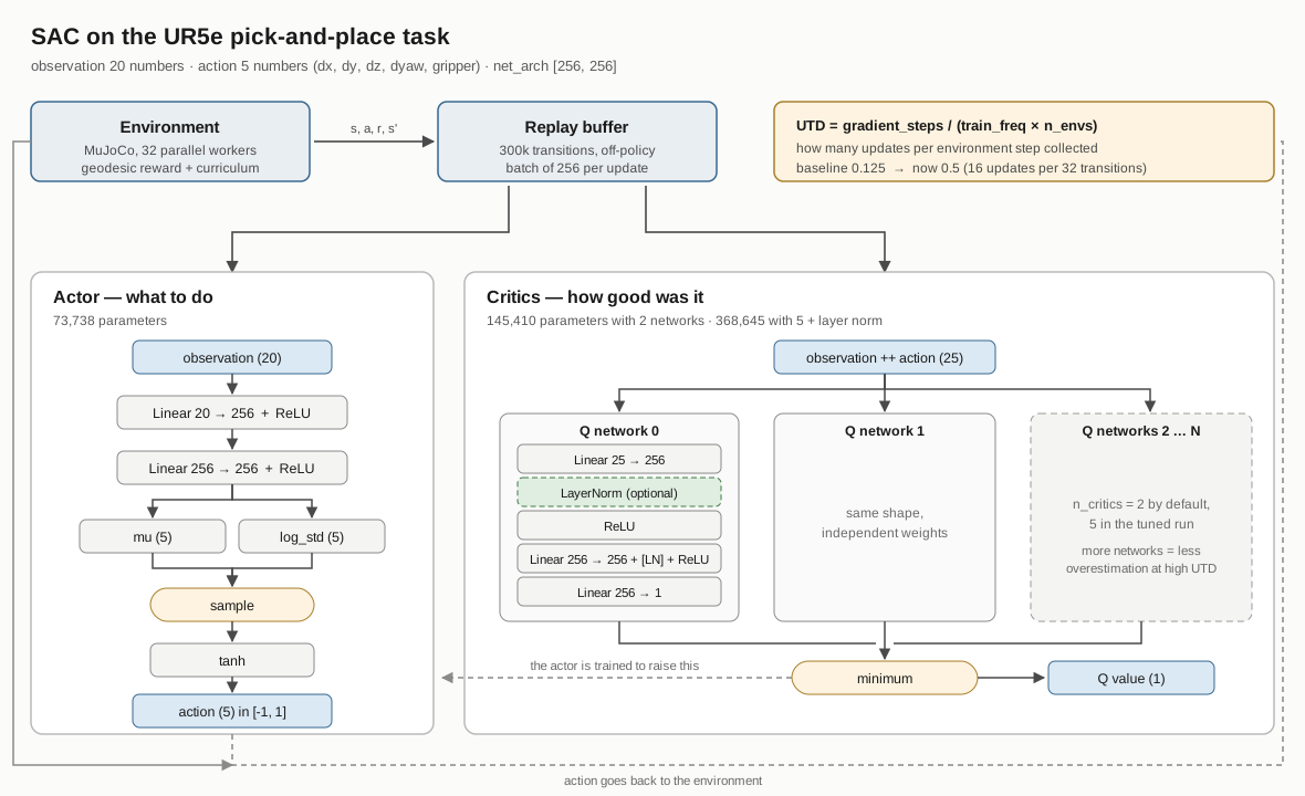
SAC with the geodesic potential and backplay curriculum solved the task from scratch in 650,000 steps, scoring 49 out of 50 on held-out seeds with an average of just 46 steps per episode.
Velocity limits and streamer faults
Because the geodesic reward contains no penalty for speed, the unconstrained SAC policy sprinted across the table at up to 0.48 m/s. While it reached 49/50 success, it triggered 40 streamer faults in 50 episodes because the Cartesian controller's acceleration safety filters tripped.
We resolved this without any retraining by tuning the Cartesian per-tick step clamp:
| Per-tick clamp | Max speed | Success | Faults | Notes |
|---|---|---|---|---|
| 0.0050 m | 0.50 m/s | 49 / 50 | 40 | Fast, but violates robot safety limits |
| 0.0025 m | 0.25 m/s | 48 / 50 | 0 | Zero faults, clean real-robot compliance |
| 0.0010 m | 0.10 m/s | 41 / 50 | 0 | Too slow; episodes timeout before reaching bin |
04Behaviour cloning: the myth of better heads
In parallel with reinforcement learning, we explored imitation learning from expert
demonstrations. Using multi-process recording, we gathered 1,000 high-quality demonstration
episodes in just 15 minutes (storing raw qpos trajectories in ~90 MB).
Standard behaviour cloning with Mean Squared Error (MSE) achieved an impressive 42/50 on our 50 held-out evaluation seeds. However, all 8 failures were compounding-drift timeouts: once the robot drifted slightly off the demonstration manifold, it never recovered.
The DAgger disaster: when the teacher lies
To address compounding error, we implemented DAgger (Dataset Aggregation): roll out the learned policy, query the expert for corrective labels on the visited states, aggregate the data, and retrain.
Unexpectedly, DAgger degraded performance across successive rounds: from 42/50 down to 24/50 in round 2, and 8/50 in round 5! Inspecting the recorded gripper labels revealed a shocking bug:
| Dataset | Mean Grip Command | % Steps with Grip > 0.4 | Mean Z Label |
|---|---|---|---|
| Original expert demonstrations | +0.451 | 72.0% | −0.057 m |
| DAgger collected labels | +0.000 | 0.0% | +0.854 m |
Across five rounds and 158,731 queried transitions, the labeller never once commanded a grasp! The replanning expert's internal state machine required the learner to come within 5 mm of its unvisited approach waypoint before advancing. Stuck in the approach phase, it commanded the gripper to stay wide open and climb toward the ceiling on every single step.
Engineering Rule: When one policy labels another policy's trajectory, always score the labeller as an autonomous driver first. If the labeller cannot drive from arbitrary off-policy states to success, it will poison the training set with consistent anti-expert demonstrations.
Do multimodal heads help?
A common critique of plain MSE in imitation learning is that regression averages conflicting demonstrations, predicting the mean of two modes (which may collide with an obstacle). To test this, we implemented and benchmarked three distinct policy heads:
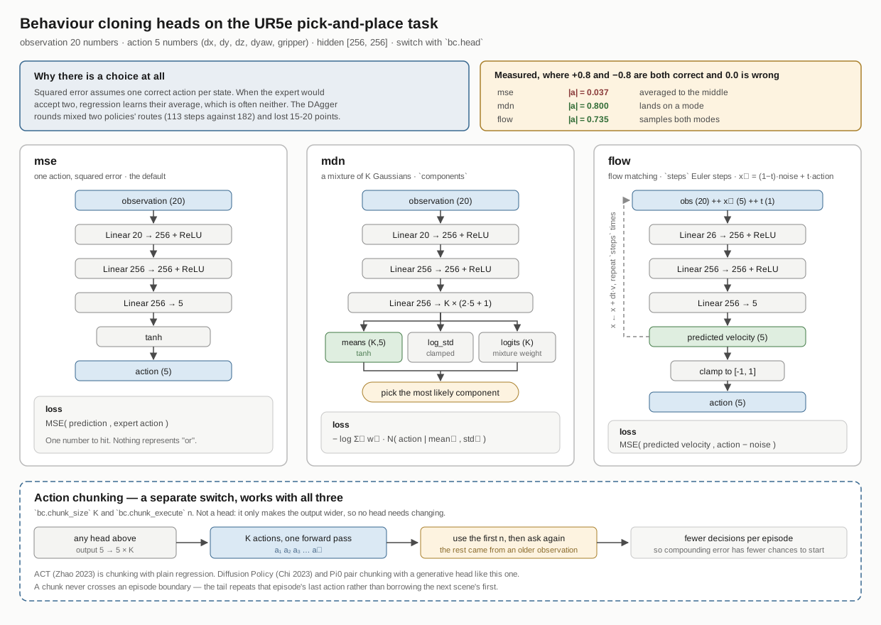
To give multimodal heads a genuine test, we created a mixed, bimodal dataset
of 306,410 transitions using two entirely different expert policies:
expert_replan (which flies low at 113 steps) and expert (which lifts
to a 20 cm travel height, taking 182 steps).
The prevailing hypothesis was that MSE would fail on the bimodal dataset by averaging the low and high paths, while MDN and Flow Matching would excel. The actual results surprised us:
| Policy Head | Single Expert (119k steps) | Bimodal Mixed Dataset (306k steps) |
|---|---|---|
| Plain MSE regression | 42 / 50 | 48 / 50 (50/50 grasped) |
| Conditional Flow Matching (CFM) | 33 / 50 | 37 / 50 |
| Mixture Density Network (MDN) | 31 / 50 | 3 / 50 |
Plain MSE actually improved from 42 to 48 on the mixed data! Why? Because the two experts diverged early, they traversed distinct regions of the state space rather than emitting conflicting actions at the same point. More data coverage outweighed head complexity. MDN collapsed because 5 Gaussian components overfitted spurious variances.
05Hitting the pixel wall
While privileged-state SAC and BC achieved 49/50 and 48/50, real robots do not receive ground-truth object XYZ coordinates from the cosmos. They have cameras.
We switched the observation to dual RGB cameras (wrist + overhead) and tested standard vision baselines. Every single one hit a brick wall:
- SAC with a CNN from scratch: 0 / 50 (1.66 million steps, never grasped).
- SAC with a frozen R3M representation: 0 / 50 (820,000 steps; linear probing showed R3M features failed to encode object Cartesian coordinates).
- SAC with ImageNet features: 0 / 50.
- Behaviour cloning with CNN (8 variants): Peaked at 11 / 50 despite spatial softmax, data augmentation, and high resolution.
Enter the VLA: fine-tuning Pi0.5
To cross the vision gap, we integrated Pi0.5 — an open-weights 3.5-billion parameter Vision-Language-Action foundation model developed by Physical Intelligence. Pi0.5 uses a flow-matching action chunking decoder conditioned on image tokens and text prompts.
Evaluating the off-the-shelf checkpoint zero-shot yielded 0/5. Supervised Fine-Tuning (SFT) on 997 demonstrations brought performance to 34/50. However, when we analyzed the remaining failures, an unmistakable pattern emerged: cubes succeeded only 10/21 times, while balls succeeded 24/29 times!
The cause was subtle: in the original demonstrations, the robot arm always began at an identical wrist orientation. The model never saw the skill of rotating its wrist to align with the flat faces of a randomly rotated cube.
We applied start-state jitter (wrist_start_jitter_rad) and gathered 7,718
demonstrations (1.63M frames, dataset pick_place_v2). Fine-tuning on this augmented
dataset propelled SFT to 47 / 50 at step 8000.
Yet even at 47/50, the last 3 failures were still cubes where the gripper fingers glanced off the edge. SFT had plateaued.
06Online RL on Pi0.5: 47/50 to 50/50 from pixels
Can online reinforcement learning in simulation take a fine-tuned 3.5B parameter VLA and correct its subtle physical failure modes?
Using RLinf (a distributed Ray-based framework for embodied RL), we implemented an environment adapter that wraps 8 parallel instances of our MuJoCo cell. The algorithm was Proximal Policy Optimization (PPO) with flow-SDE exploration noise and a learned value head.
Crucially, the reward was pure sparse binary task outcome: +1.0 if the object lands in the bin, and 0.0 otherwise. No geodesic potential, no shaped bonuses, and no privileged object coordinates whatsoever!
The rendering bottleneck
On our cluster's NVIDIA H200 GPUs, the first PPO run took an excruciating 21 minutes per training step — with 96% of the wall clock spent waiting for MuJoCo to render 224×224 camera frames. MuJoCo's default cell model requested an 8192×8192 shadow map, which severely stalled Hopper's compute-optimized graphics pipeline (0.16 s/frame vs. 0.011 s on a desktop RTX 3080).
By reducing the rollout shadow map to 2048 (which differed from 8192 on fewer than 0.7% of edge pixels) and rendering only at action chunk boundaries, training time plummeted from 21 minutes down to 5.3 minutes per step.
In just 60 to 80 PPO steps (under 9 hours on a single H200 GPU), Pi0.5 achieved a perfect 50/50 score on our held-out EVAL_ID test seeds, completely eliminating the cube grasp defect!
What online PPO actually changed
| Metric | SFT Step 8000 (Start) | RL Step 60 | RL Step 80 |
|---|---|---|---|
| Overall Held-Out Success | 47 / 50 | 50 / 50 | 50 / 50 |
| Cube Grasps | 19 / 21 | 21 / 21 (100%) | 21 / 21 (100%) |
| Sphere Grasps | 28 / 29 | 29 / 29 (100%) | 29 / 29 (100%) |
| Mean Episode Steps | 188 steps | 155 steps | 147 steps (−22%) |
| Streamer Controller Faults | 0 | 0 | 0 |
Under PPO, the policy did not just patch the cube grasp — it also learned to execute the entire trajectory 22% faster. Because discounting ($\gamma = 0.99$) pays for earlier completion, PPO pruned unnecessary pauses during the approach and transport phases while keeping Cartesian accelerations well within the controller's safety threshold.
07Stress-testing across 16 abnormal scenarios
Laboratory benchmarks often measure success in pristine environments. Real-world factories and hospitals feature smeared lenses, flickering lights, shadows, occlusions, and varying surface friction.
To evaluate true robustness, we built an automated Scenario Engine incorporating 16 out-of-distribution stress tests scored across 50 seeds each (800 evaluation episodes in total):
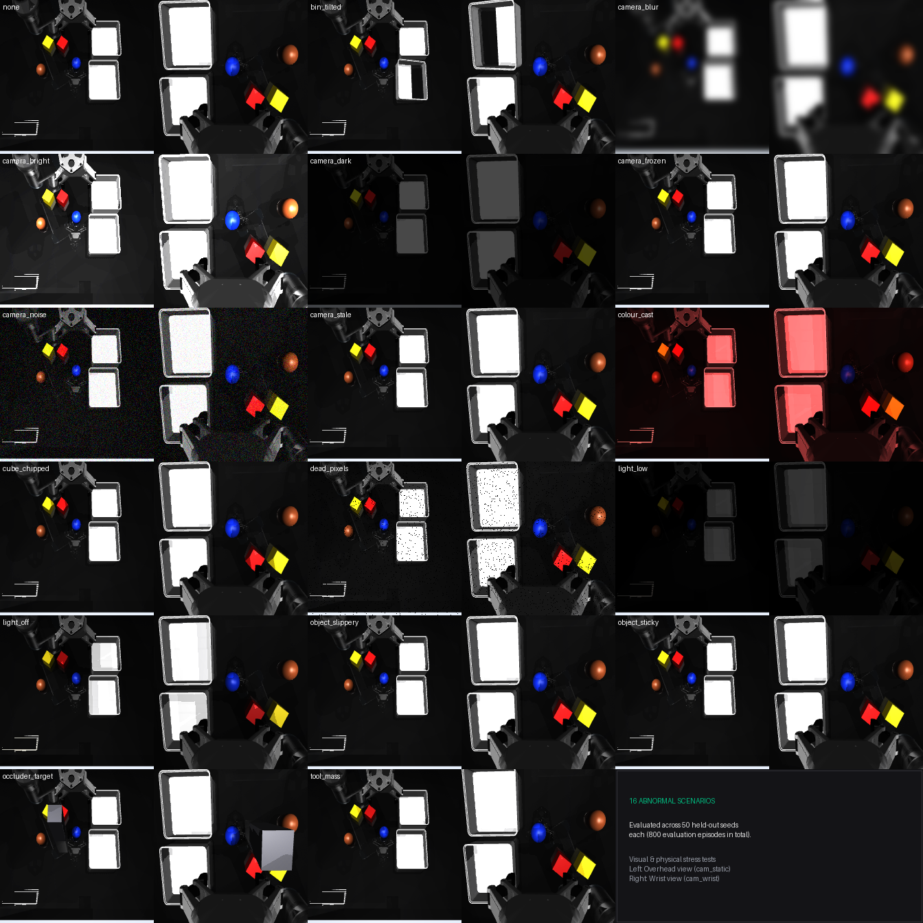
Finding 1: Plain RL provides free visual robustness
Our first surprise came when evaluating the plain PPO model (RL step 80), which had been trained exclusively in the pristine simulation. Its summed score across all 16 scenarios jumped from 596 to 624!
Why? A more precise, confident motor policy tolerates noisier visual inputs. Gains were especially pronounced on colour casts (38 → 47), overhead lights turned off (40 → 47), and slippery objects (41 → 48).
Finding 2: RL alone cannot fix broken visual representations
However, two visual scenarios remained completely broken under plain RL: camera blur (only 5/50) and frozen camera (0/50).
We attempted to train RL directly on the scenarios. It completely failed to improve blur (5/50 remained 5/50). The reason is sample efficiency: the RL update budget is approximately 1/40th of the SFT pretraining budget. While RL has ample gradient to nudge a motor action, it cannot reconstruct deep visual feature extractors from scratch under a sparse binary reward.
Finding 3: Data fixes perception; RL fixes control
To fix perception, we modified our data export pipeline to render one-third of our demonstration
dataset under randomized visual scenarios. This produced dataset pick_place_v3
(11,454 demonstrations, 2.54 million frames).
Fine-tuning Pi0.5 on pick_place_v3 immediately unlocked blur perception:
camera blur success leaped from 4 to 34 out of 50!
Finally, we ran online PPO on top of this augmented checkpoint with a 50% scenario mix. The combined model set the state of the art across almost every condition:
| Scenario | SFT 8000 | RL Step 80 | SFT v3 | SFT v3 + PPO (150 steps) |
|---|---|---|---|---|
| Pristine clean cell | 48 / 50 | 50 / 50 | 47 / 50 | 50 / 50 |
| Camera blur (2–5 px) | 4 / 50 | 5 / 50 | 34 / 50 | 42 / 50 |
| Camera sensor noise | 27 / 50 | 34 / 50 | 33 / 50 | 45 / 50 (49/50 in v3rl2) |
| Low lighting | 36 / 50 | 40 / 50 | 41 / 50 | 47 / 50 |
| Overhead light off | 40 / 50 | 47 / 50 | 45 / 50 | 47 / 50 |
| Dead sensor pixels | 37 / 50 | 45 / 50 | 39 / 50 | 48 / 50 |
| Extreme bright exposure | 42 / 50 | 45 / 50 | 45 / 50 | 50 / 50 |
| Sticky object dynamics | 42 / 50 | 45 / 50 | 44 / 50 | 49 / 50 |
| 16-Scenario Sum (max 800) | 596 | 624 | 641 | 699 / 800 |
Interactive Scenario Rollouts
Each video below compares the baseline pristine execution against the stressed scenario side by side (Left: Overhead camera, Right: Wrist camera). Select a scenario tab to watch the full-resolution rollout:
What remains unsolved
Two scenarios did not yield:
- Frozen camera (4 / 50): Pi0.5 processes single-timestep image frames without recurrent history or frame stacking. To a memoryless model, a frozen video feed looks like an unchanging world. Solving this requires temporal sequence conditioning.
- Target occluder (32 / 50): When an obstacle physically blocks the target, a simple pick-and-place policy cannot clear the blocker first. This requires interactive multi-stage task planning.
08Master scoreboard
Every method evaluated on the exact same 50 held-out seeds under identical physics:
| Approach | Inputs | Held-Out Score | Key Failure Mode / Notes |
|---|---|---|---|
| Scripted Expert | Ground truth poses | 50 / 50 (100%) | Demonstration source; 0 streamer faults |
| SAC dense reward from scratch | 20 numbers (state+task) | 0 / 50 (0%) | Hovered beside object to exploit per-step proximity |
| PPO geodesic from scratch | 20 numbers (state+task) | 0 / 50 (0%) | Failed to explore diverse initial configurations |
| SAC geodesic + curriculum | 20 numbers (state+task) | 49 / 50 (98%) | Fastest policy (46 steps); solved in 650k env steps |
| Behaviour cloning (MSE) | 20 numbers (state+task) | 48 / 50 (96%) | 50/50 grasped; 306k demo steps |
| Behaviour cloning (Flow Matching) | 20 numbers (state+task) | 37 / 50 (74%) | High sample quality but slower inference |
| Behaviour cloning (MDN) | 20 numbers (state+task) | 3 / 50 (6%) | Mixture modes collapsed on bimodal data |
| SAC / BC from pixels (CNN/R3M) | Dual RGB cameras | 0 / 50 (0%) | Failed to ground spatial coordinates from scratch |
| Pi0.5 zero-shot (Franka weights) | Dual RGB + text | 0 / 5 (0%) | Kinematic mismatch across embodiments |
| Pi0.5 SFT v1 (997 demos) | Dual RGB + text | 34 / 50 (68%) | Wrist yaw bias: cubes failed 10/21 |
| Pi0.5 SFT v2 (7,718 jittered demos) | Dual RGB + text | 47 / 50 (94%) | Cube grasp edge-hits remained |
| Pi0.5 SFT v2 + PPO (sparse reward) | Dual RGB + text | 50 / 50 (100%) | Cube grasps 21/21; 22% faster; 0 controller faults |
| Pi0.5 SFT v3 + PPO (scenario mix) | Dual RGB + text | 699 / 800 (87.4%) | Robust across 16 abnormal visual and physical scenarios |
09Seven engineering lessons
- Proximity reward shaping over long horizons is dangerous: Rewarding being near a goal pays an agent for doing nothing. Reward must measure directional progress ($\phi_{\text{prev}} - \phi$).
- Profile before optimizing execution speed: We initially blamed arm velocity for long 700-step episodes. Profiling revealed that 503 of 724 steps were spent waiting for the gripper fingers to close on a cube. Moving the arm 4x faster only produced overshoot and controller faults.
- Always evaluate labellers as standalone drivers: When implementing DAgger, test the labeller policy by letting it drive the robot autonomously. Our labeller suffered from state-machine lockup, silently commanding anti-expert actions for five entire rounds.
- Data coverage beats fancy policy heads: In behaviour cloning, plain MSE regression on 306k demonstration steps outperformed complex Flow Matching and Mixture Density heads. Don't add generative complexity before maximizing dataset diversity.
- Pretrained representations make vision tractable: Scratch CNNs and frozen out-of-domain encoders (R3M, ImageNet) scored 0%. A foundation VLA (Pi0.5) provided the spatial grounding necessary to learn from vision.
- RL fine-tunes motor control, not visual feature extractors: RL under sparse reward lacks the sample budget to learn visual representations from blurred frames. Augment data in SFT to fix perception; use RL to perfect physical precision.
- Data-centre GPUs hate shadow maps: An NVIDIA H200 took 0.16 s to render an 8192 shadow map in MuJoCo. Lowering shadow maps to 2048 and rendering only at action chunk boundaries reduced training step wall-time by 75%.
Code and reproduction
The entire simulation environment, scripted expert, evaluation suites, and training configurations are open source:
To evaluate the 50/50 Pi0.5 + PPO checkpoint on the 50 held-out evaluation seeds:
# In the RLinf environment with GPU rendering:
MUJOCO_GL=egl python3 scripts/run_rollouts.py \
    --config-name scenario_eval \
    env.scenario=null \
    run.checkpoint=~/RLinf/storage_local/urvla_outputs/.../global_step_150/ \
    run.episodes=50
To run the hand-written expert or train the privileged-state SAC policy:
# 1. Verify the cell contract (12 checks)
python3 scripts/check_env.py

# 2. Score the 50/50 expert demonstrator
python3 scripts/run_rollouts.py --config-name expert

# 3. Train SAC with geodesic potential & backplay curriculum
python3 scripts/train_rl.py --config-name sac_geodesic_curriculum_utd
References
Physical Intelligence et al. (2024). “π0: A Vision-Language-Action Flow Model for General Robot Manipulation.” arXiv:2410.24164.
Todorov, E., Erez, T., & Tassa, Y. (2012). “MuJoCo: A physics engine for model-based control.” IEEE/RSJ International Conference on Intelligent Robots and Systems (IROS).
Haarnoja, T., Zhou, A., Abbeel, P., & Levine, S. (2018). “Soft Actor-Critic: Off-Policy Maximum Entropy Deep Reinforcement Learning with a Stochastic Actor.” International Conference on Machine Learning (ICML).
Schulman, J., Wolski, F., Dhariwal, P., Radford, A., & Klimov, O. (2017). “Proximal Policy Optimization Algorithms.” arXiv:1707.06347.
Ross, S., Gordon, G., & Bagnell, D. (2011). “A Reduction of Imitation Learning and Structured Prediction to No-Regret Online Learning.” AISTATS.